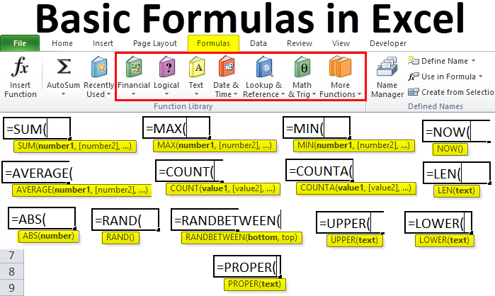
Excel Jobs - The Facts

By pressing ctrl+change+center, this will certainly compute and also return worth from numerous ranges, as opposed to simply individual cells added to or multiplied by each other. Determining the amount, item, or ratio of individual cells is simple-- just make use of the =AMOUNT formula and also get in the cells, worths, or variety of cells you desire to do that math on.

If you're aiming to discover total sales profits from a number of sold systems, for instance, the array formula in Excel is ideal for you. Here's just how you 'd do it: To start utilizing the array formula, type "=SUM," and in parentheses, enter the first of two (or three, or four) arrays of cells you want to increase together.

This represents reproduction. Following this asterisk, enter your 2nd variety of cells. You'll be increasing this second variety of cells by the initial. Your development in this formula should now appear like this: =AMOUNT(C 2: C 5 * D 2:D 5) Ready to press Enter? Not so quickly ... Since this formula is so difficult, Excel reserves a various key-board command for arrays.

This will certainly recognize your formula as an array, covering your formula in support characters and also effectively returning your item of both varieties integrated. In revenue estimations, this can reduce your effort and time dramatically. See the last formula in the screenshot over. The MATTER formula in Excel is represented =MATTER(Start Cell: End Cell).

As an example, if there are 8 cells with gotten in worths between A 1 as well as A 10, =COUNT(A 1: A 10) will return a value of 8. The COUNT formula in Excel is specifically useful for big spreadsheets, where you intend to see the number of cells have real entries. Do not be deceived: This formula will not do any math on the worths of the cells themselves.

The Ultimate Guide To Countif Excel

Making use of the formula in vibrant above, you can easily run a matter of active cells in your spread sheet. The result will look a little something like this: To execute the average formula in Excel, enter the worths, cells, or series of cells of which you're determining the average in the style, =STANDARD(number 1, number 2, etc.) or =STANDARD(Begin Worth: End Worth).

Discovering the standard of a variety of cells in Excel keeps you from needing to discover specific amounts and also after that carrying out a separate division formula on your total amount. Using =AVERAGE as your initial message entry, you can let Excel do all the job for you. For referral, the standard of a group of numbers is equal to the sum of those numbers, separated by the variety of things because group.

This will certainly return the amount of the worths within a desired variety of cells that all meet one standard. For instance, =SUMIF(C 3: C 12,"> 70,000") would certainly return the sum of values in between cells C 3 as well as C 12 from just the cells that are greater than 70,000. Allow's claim you want to identify the revenue you produced from a checklist of leads who are linked with certain area codes, or determine the amount of certain workers' wages-- however only if they fall over a certain amount.

With the SUMIF function, it does not have to be-- you can easily add up the amount of cells that satisfy certain criteria, like in the income example above. The formula: =SUMIF(variety, criteria, [sum_range] Range: The range that is being tested using your requirements. Standards: The requirements that determine which cells in Criteria_range 1 will be totaled [Sum_range]: An optional array of cells you're mosting likely to include up in addition to the initial Variety entered.

In the example listed below, we wished to determine the sum of the wages that were above $70,000. The SUMIF function built up the dollar quantities that exceeded that number in the cells C 3 through C 12, with the formula =SUMIF(C 3: C 12,"> 70,000"). The TRIM formula in Excel is signified =TRIM(message).

Vlookup Excel for Dummies

As an example, if A 2 consists of the name" Steve Peterson" with undesirable areas prior to the given name, =TRIM(A 2) would return "Steve Peterson" without rooms in a brand-new cell. Email and also submit sharing are wonderful tools in today's office. That is, till among your coworkers sends you a worksheet with some truly fashionable spacing.

Instead of fastidiously eliminating and also adding rooms as needed, you can clean up any uneven spacing using the TRIM feature, which is made use of to remove extra areas from data (other than for single areas between words). The formula: =TRIM(message). Text: The text or cell where you intend to remove areas.

To do so, we went into =TRIM("A 2") into the Formula Bar, and reproduced this for each name below it in a new column beside the column with unwanted spaces. Below are a few other Excel solutions you may discover helpful as your information monitoring requires expand. Allow's state you have a line of text within a cell that you wish to break down into a couple of various segments.

Function: Used to remove the first X numbers or personalities in a cell. The formula: =LEFT(text, number_of_characters) Text: The string that you wish to extract from. Number_of_characters: The number of characters that you desire to draw out beginning with the left-most character. In the example listed below, we went into =LEFT(A 2,4) right into cell B 2, and also duplicated it into B 3: B 6.

Purpose: Used to remove characters or numbers between based on position. The formula: =MID(text, start_position, number_of_characters) Text: The string that you want to draw out from. Start_position: The placement in the string that you desire to begin extracting from. For example, the initial placement in the string is 1.

Excel Formulas Things To Know Before You Buy

In this example, we entered =MID(A 2,5,2) into cell B 2, and also copied it right into B 3: B 6. That enabled us to draw out both numbers beginning in the 5th setting of the code. Function: Used to remove the last X numbers or personalities in a cell. The formula: =RIGHT(message, number_of_characters) Text: The string that you wish to extract from.

excel formula year from date excel formulas today's date formula excel odd even